CityHiker

In my last post, I described in detail the challenges of optimizing geospatial data APIs. From the beginning, one of the features I wanted to support was the idea of pathfinding. If you want to avoid a hill, one way to do that is with a top-down view of steep roads around you. This gives you an easy way to decide for yourself where you want to go. We can provide that with a line segment overlay. Another way is to find a path automagically, given a specific goal.

Pathfinding is Hard

Finding a path through a set of unstructured line segments is very computationally expensive. A graph would be much easier to work with. If we’re going to consider a graph, we must first convert the line segment data into a graph representation. Then, we can consider strategies for finding and evaluating possible paths. First, let’s look at the construction of the graph.

Graph Construction

Graphs are made up of nodes and edges. Starting at the lowest level, line segment data is, in essence, a set of unconnected edges. Each segment is isolated as individual records in a database. In order to generate the full graph, we need to build a set of nodes from the line segment endpoints and connect them.

Discrete Grid

Following the same discrete grid strategy from before, we can convert all the lat/lng floating-point values to 26-bit signed integer values. This defines a minimum grid size of one meter, and any values falling within a grid cell will coalesce into the same cell. It’s ok to have more than one segment sharing a location. These represent intersections in the graph. It’s clear we will need to use some filtering. This discretization acts as our first filtering mechanism for reducing the total number of nodes required to represent the surrounding area.

Clustered Caching for Duplicate Consolidation

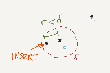
CityHiker’s line segment data is derived from OpenStreetMap data. Since they rely heavily on crowdsourced data, there is often data duplication. Discrete grids help to reduce the raw data size. Beyond that, we can rely on a clustered cache strategy for node insertion into the graph. As each node is inserted, the cache attempts to find an existing node nearby the input. If one exists, the existing one is used instead.

Consider this pseudoSQL:

// given lat0, lng0, threshold
find node 
  where abs(latitude-lat0) < threshold 
  and abs(longitude-lng0) < threshold
  limit 1

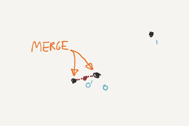
If this returns anything, the location coordinate from the resulting node is used instead of the input (lat0, lng0) value. Observant readers will note this represents data loss. Advanced topics include rolling average computation, based on the average of locations of the clustered nodes. In order to support that, we would need to add a field to Node to represent the total number of aggregated points averaged into the current value. That way, we can update the node location as follows:

latitude = (latitude * numAggregatedPoints + lat0) / (numAggregatedPoints + 1)
longitude = (longitude * numAggregatedPoints + lng0) / (numAggregatedPoints + 1)
numAggregatedPoints += 1

This introduces an error delta for each point, but the delta is minimized for the set of points, by virtue of the rolling average. This isn’t strictly necessary, but it does offer an improvement over the strategy using only the initial point.

Complexity

Without the cache, insert operations have time complexity of typically O(1) or at worst O(log n). Using a clustered cache approach, the time complexity increases to O(n). Every time we insert a node, we must check every node for proximity. The value of n is potentially different in both cases, constrained by the specific details in the set of line segments. Disparate sets of unconnected line segments will have large values of n, whereas fully connected sets will have smaller values.

Path Generation

Once we have our nodes and edges, with all nodes clustered within a threshold, we can begin to find paths matching our input configuration. CityHiker asks the user for a total path distance and a easy/medium/hard selector. We also need to define constraints that apply to all paths, regardless of user preference. For example, we assume paths must be complete loops, where the start and end node are the same.

Strategy

First, we traverse the graph outward from the start node, finding all paths with distance of about half the total. In other words, we work with a set of incomplete paths, extending them until the resulting path length is within a threshold of the desired distance. From those paths, we extract a small set, attempting to select paths whose end nodes are uniformly distributed around the start. Paths with no valid extension are removed from the set.

For each of those outbound paths, we attempt to find a path back to the start node from the path end node. We combine the paths to form a loop and then order the resulting set to find the best match for easy/medium/hard preference. All options are displayed to the user in a list, giving them the option to choose. The results should be random each time.

Validation

This algorithm may not identify a return path for all of the outbound paths. We must consider this as part of the design. By selecting a larger number of paths in the initial filter, we improve the chances of multiple outbound paths with valid matching return paths. Additionally, we may encounter situations where the resulting paths do not satisfy the easy/medium/hard filter. If the results are sufficiently random, we can simply retry if we don’t get results on the first attempt.